Neural Network Radial Based Function (RBF) approach in
pridicting of material removal rate and surface roughness in electrical discharge machining
Morteza Sadegh Amalnik,
Farzad Momeni,
Computer and
Automation R&D Center of ACECR-Sharif Branch,
Department of Mechanical and Industrial
Engineering, University of Qum and
Tabriz, Iran
Abstract
This paper uses Radial Based Function(RBF)
Artificial Neural Network(ANN) approach for prediction of material removal rate
and surface roughness and presents the results of the experimental
investigation. Charmilles Technology (EDM-Robofil machine) in the mechanical
engineering department is used for machining parts. The networks have four inputs of current (I),
voltage (V), Period of pulse on (Ton) and period of pulse off (Toff)
as the input processes variables. Two outputs results of material removal rate
(MRR) and surface roughness (Ra) as performance characteristics. In order to
train the network, and capabilities of the models in predicting material removal
rate and surface roughness, experimental data are employed. Then the output of
MRR and Ra obtained from RBF neural net compare with experimental
results, and amount of relative error is calculated.
Keywords:
Electro-discharge machining (EDM), Artificial Neural Networks (ANN), RBF
Introduction:
Electro-discharge machining (EDM) is
non-conventional, process, which erodes material from the work piece by a
series of discrete sparks between a work-piece and tool electrode immersed in a
liquid dielectric medium [1]. Operation and process planning, parametric
analysis, verification of the experimental results, and improving the process
performance by implementing/incorporating some of the theoretical findings [2].
A systematic study of the phenomenon of the electrical discharge in a liquid
dielectric has proven to be very difficult due to its complexity. The erosion
by an electric discharge involves phenomena such as heat conduction, melting,
evaporation, ionization, formation, and collapse of gas bubbles and energy
distribution in the discharge channel. These complicated phenomena coupled with
surface irregularities of electrodes, interactions between two successive
discharges, and the presence of debris particles make the process too abstruse,
so that complete and accurate physical modeling of the process has not been
established yet [3,4]. There are a lot of theoretical studies concerned with
microscopic metal removal arising from a single spark, the effects being
modeled from heat conduction theory [5,6,7and 8]. Recent established models for
EDM are mainly based on empirical data or basically data driven models.
Ghoreishi and Atkinson [9, 10] employed statistical modeling and process
optimization for the case of EDM drilling and milling. Wang and Tsai [11, 12]
proposed semi-empirical models of the material removal rate, surface finish and
tool wear on the work and the tool for various materials in EDM, employing
dimensional equations based on relevant process parameters for the screening
experiments and the dimensional analysis. Artificial neural networks (ANNs), as
one of the most attractive branches in artificial intelligence, has the
potentiality to handle problems such as modeling, estimating, prediction,
diagnosis, and adaptive control in complex non-linear systems [13]. The
capabilities of ANNs in capturing the mathematical mapping between input
variables and output features are of primary significance for modeling
machining processes. The use of neural networks in both EDM and wire-EDM
(WEDM) processes has also been reported. Kao and Tamg [14]. Liu and Tamg [15]
have employed feed forward neural networks with hyperbolic tangent functions
and abductive networks for the classification and on-line recognition of
pulse-types. Based on their results, discharge pulses have been identified and
then used for controlling the EDM machine. Indurkhya and Rajurkar [16]
developed a 9-9-2-size back propagation neural network for orbital EDM
modeling. Spedding and Wang [17, 18], and Tamg et al. [19] have developed BP neural
networks for modeling of WEDM. Experimental results have shown that the cutting
performance of WEDM can be greatly enhanced using the neural model. Tsai and
Wang [20] have been presented seven models for predictions of surface finish
and material removal rate of work in EDM process.
1.
Artificial neural network models of the EDM process
In the
current work, three supervised neural networks for modeling the EDM process are
compared. The first one is a Logistic Sigmoid Multi-layer Perceptron (LOGMLP);
the Second is a Hyperbolic Tangent sigmoid Multi-layer Perceptron (TANMLP) and
third is a Radial Basis Network (RBN) with Gaussian activation functions. The
LOGMLP and TANMLP are two different BP neural networks. The LOGMLP is a Back
propagation neural network with log-sigmoid transfer function in hidden layer
and output layer, but the TANMLP is a Back propagation neural network with
tangent-sigmoid transfer function in hidden layer and output layer. The BP
Neural Network is very popular, especially in the area of manufacturing
modeling, as its design and operation are relatively simple. The radial basis
network has some additional advantages such as rapid convergence and less error.
In particular, most commonly used RBNs involve fixed basis functions with
linearly appearing unknown parameters in the output layer. Radial Basis
networks may require more neuron than standard feed-forward back propagation
networks, but often they can be designed in a fraction of the time it takes to
train standard feed-forward networks. They work best when many training vectors
are available. It is commonly known that linearity in parameters in RBN allow
the use of least squares error based updating schemes that have faster
convergence than the gradient-descent methods used to update the nonlinear
parameters of multi-layer BP ANN. In practice, the number of parameters in RBN
starts becoming unmanageably large only when the number of input features increases
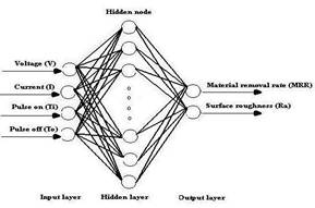
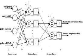
beyond about 10 or 20, which is not the case in our study. Hence, the use of
RBN was practically possible for our problem. The general input and output for
RBFNN is demonstrated in figure(1) and figure(2). MATLAB Neural Network Tool Box was used as a
platform to create the networks.
|
|
|
|
Figure1.Input
and output neural network with one
hidden layer |
Figure2.
Architecture of the RBFN. |
2.
Experimental details
In order to
obtain different machining process parameters and output features for training
and testing of neural networks, a series of experiments was performed on a
ROBOFORM 200 machine. At first, some preliminary tests were carried out to
determine the stable domain of the machine parameters and also the different
ranges of process variables. Based on preliminary tests results and working
characteristics of the EDM machine, discharge current (I), period of pulse on
(Ti), Period of pulses off (To) and source voltage (V) were chosen as
independent input parameters. During these experiments, by altering the values
of the input parameters in different levels, stable states of the machining
conditions have also been specified.
Accordingly, the experiments were
conducted with three levels of discharge current, three levels of period of
pulses on, three levels of period of pulses off and three levels of source
voltage. Table 1 shows the input process variables and their levels in the
experiments.
Throughout
the experiments, SPK steel and commercial copper was used as work-piece and
tool electrode materials. Also, the dielectric fluid used was elf oil.
Particular attention was paid to ensuring that operating conditions permitted.
Effective flushing of machining debris
from the working region. Thus, the experiments were done in the planning
process mode in which the bottom surface of the electrode is flat and parallel
to the work-piece surface. Also, the diameter of cylindrical electrode was
equal to the diameter of the round bar work-piece and was chosen to be 12 mm.
The total data obtained from machining experiments (3*3*3*3) is 81 and these
forms the neural networks' training and testing sets. To achieve validity and
accuracy, each test was repeated three times. Material removal rate (MRR) and
surface roughness (Ra) were assigned as performance characteristics or process
outputs, since the performance of any machining process is evaluated in terms
of these two measures. Then, the mean values of the three response measurements
(MRR and Ra) were used as output at each set of parameters. The machining time
considered for each test was dependent on the discharge current and much time
was allocated to the tests with lower current. The material removal rate (MRR)
was estimated by weighing the work-piece on a digital single pan balance before
and after the experiments and was reported in gr/hr unit. The surface roughness
(Ra) was measured by means of a Mahr with Ra value in microns at a cut-off
length of 0.8 mm.
Table 1.
Pertinent process parameters and their levels for machining experiments.
|
Process
parameters |
Operating conditions |
|
Source
voltage V (v) |
80,160,200 |
|
Discharge
current I (A) |
6,16,48 |
|
Period of pulses on
Ti ( |
6.4,100,800 |
|
Period of
pulses off To ( |
12.8,50,400 |
For
normalization of input and output variable, the following linear mapping
formula is used:
![]()
Modeling of
EDM process with RBF network are composed of two stages: training and testing
of the networks with experimental machining data. The training data consisted
of values for current (I), period of pulses on (Ti), period of pulses off (To),
and source voltage (V), and the corresponding material removal rate (MRR) and
surface roughness (Ra). In all, 81 such data sets were used, of which 66 data
sets were selected at random and used for training purposes while the remaining
15 data sets were presented to the trained networks as new application data for
verification (testing) purposes. Thus, the networks were evaluated using data
that had not been used for training.
In RBF
neural network, two parameters need to be defined. Spread factor and goal factor.
The spread factor S, has to be
specified depending on the particular case in hand. It has to be smaller than
the highest limit of the input data and larger than the lowest limit [20].
Based on this, and assuming that all the training data is mapped between -1 and
1. The goal factor value is set to zero, since error is a decisive factor in
this study. Table 2 shows the 15 experimental data sets, which are used for
verifying or testing network capabilities in modeling the process. Therefore,
the general network structure is supposed to be 4-n-2, which implies 4 neurons
in the input layer, n neurons in the hidden layer, and 2 neurons in the output
layer. Then, by varying the number of hidden neurons and spread factor,
different network configurations are
trained, and their performances are checked. The results are shown in table
3.1, 3.2 and 3.3.
3.
Results
3.1.
Training results
Each
experimental set (except the validation set) is used to train each network.
This training is repeated for each topology. The performance is measured by the
linear regression (R) of each
output. With this analysis it is possible to determine the response of the
network with respect to the targets. A value of 1 indicates that the network is
perfectly simulating the training set while 0 means the opposite. For all the
cases in this study, the value of R (for
all output sets) is shown in Table 5. The case of RBN showed a good fitting
pattern for all the cases) as expected since the goal error factor is set to
zero.
3.2.
Validation results of the LOGMLP, TANMLP and RBF model
As a
result, from table 3.1, the best network structure of BP model is picked to
have 10 neurons in the hidden layer with the average verification errors of
20.31% and 5.13% in predicting MRR and Ra, respectively, for TANMLP. Thus, it
has a total average error of 12.72% over the 15 experimental verification data
sets. And from table 3.2, the best network structure of BP model is picked to
have 11 neurons in the hidden layer with the average verification errors of
32.02% and 12.91% in predicting MRR and Ra, respectively, for LOGMLP. Thus, it
has a total average error of 22.47% over the 15 experimental verification data
sets. As a result, from table 3.3, the best network of RBF model is picked to
have 66 neurons in hidden layer, while spread factor is 0.07.The average
verification errors of 17.54% and 7.84% in predicting MRR and Ra, respectively.
Thus it has a total error of 12.69% over the 15 experimental verification data
test. Table 4.1,4.2 and 4.3 shows the comparison of experimental and predicted
values for MRR and Ra in verification cases by three neural network models.
Table
2. Machining conditions for verification experiments
|
V (v) |
I (A) |
Ti ( |
To( |
MRR
(gr/hr) |
Ra( |
|
80 |
6 |
6.4 |
400 |
0.2 |
2.62 |
|
80 |
6 |
800 |
12.8 |
0.3 |
2.87 |
|
80 |
16 |
6.4 |
400 |
0.3 |
3.05 |
|
80 |
16 |
800 |
12.8 |
10.0 |
7.63 |
|
80 |
48 |
100 |
12.8 |
63.0 |
9.75 |
|
160 |
6 |
800 |
12.8 |
0.2 |
2.68 |
|
160 |
16 |
100 |
12.8 |
20.4 |
8.32 |
|
160 |
16 |
800 |
50 |
12.8 |
7.85 |
|
160 |
48 |
100 |
12.8 |
55.1 |
9.31 |
|
160 |
48 |
800 |
400 |
44.0 |
10.61 |
|
200 |
6 |
6.4 |
400 |
0.3 |
2.05 |
|
200 |
6 |
800 |
50 |
0.3 |
2.69 |
|
200 |
16 |
100 |
12.8 |
21.6 |
8.32 |
|
200 |
48 |
6.4 |
12.8 |
7.6 |
4.27 |
|
200 |
48 |
800 |
50 |
54 |
10.43 |
|
Test No. |
V (v) |
I (A) |
Ti ( |
To( |
MRR
(gr/hr) |
Ra( |
|
1 |
80 |
6 |
6.4 |
400 |
0.2 |
2.62 |
|
2 |
80 |
6 |
800 |
12.8 |
0.3 |
2.87 |
|
3 |
80 |
16 |
6.4 |
400 |
0.3 |
3.05 |
|
4 |
80 |
16 |
800 |
12.8 |
10.0 |
7.63 |
|
5 |
80 |
48 |
100 |
12.8 |
63.0 |
9.75 |
|
6 |
160 |
6 |
800 |
12.8 |
0.2 |
2.68 |
|
7 |
160 |
16 |
100 |
12.8 |
20.4 |
8.32 |
|
8 |
160 |
16 |
800 |
50 |
12.8 |
7.85 |
|
9 |
160 |
48 |
100 |
12.8 |
55.1 |
9.31 |
|
10 |
160 |
48 |
800 |
400 |
44.0 |
10.61 |
|
11 |
200 |
6 |
6.4 |
400 |
0.3 |
2.05 |
|
12 |
200 |
6 |
800 |
50 |
0.3 |
2.69 |
|
13 |
200 |
16 |
100 |
12.8 |
21.6 |
8.32 |
|
14 |
200 |
48 |
6.4 |
12.8 |
7.6 |
4.27 |
|
15 |
200 |
48 |
800 |
50 |
54 |
10.43 |
Table3.1.The
effects of different number of hidden neurons on the TANMLP
|
(No.
Of hidden neuron |
Epoch |
Average
error in MRR (%) |
Average
error in Ra (%) |
Total
average error (%) |
|
8 |
1529 |
43.59 |
6.47 |
25.03 |
|
9 |
1042 |
28.44 |
7.22 |
17.83 |
|
10 |
1137 |
20.31 |
5.13 |
12.72 |
|
11 |
2076 |
35.47 |
8.44 |
21.96 |
Table3.2.The
effects of different number of hidden neurons on the LOGMLP
|
No. Of
hidden neuron |
Epoch |
Average
Error in MRR (%) |
Average Error in
Ra (%) |
Total
Average Error (%) |
|
6 |
7437 |
36.42 |
10.45 |
23.44 |
|
7 |
1244 |
42.28 |
9.23 |
25.76 |
|
8 |
334 |
48.72 |
10.60 |
29.66 |
|
9 |
572 |
37.61 |
14.48 |
26.05 |
|
10 |
311 |
75.14 |
12.18 |
43.66 |
|
11 |
848 |
32.83 |
12.91 |
22.87 |
|
15 |
542 |
67.54 |
9.31 |
38.43 |
Table 3.3.
The effects of different spread factor on the RBF model (Radial Basis Network)
|
Spread
factor |
Average Error in MRR (%) |
Average Error in
Ra (%) |
Total Average Error (%) |
|
0.01 |
21.00 |
7.41 |
14.21 |
|
0.03 |
20.81 |
7.17 |
13.99 |
|
0.05 |
20.54 |
7.23 |
13.89 |
|
0.06 |
19.48 |
7.41 |
13.45 |
|
0.07 |
17.54 |
7.84 |
12.69 |
|
0.08 |
20.87 |
9.02 |
14.95 |
|
0.09 |
24.98 |
10.28 |
17.63 |
|
0.1 |
28.17 |
11.51 |
19.84 |
|
0.12 |
35.85 |
13.66 |
24.76 |
|
0.15 |
46.04 |
16.01 |
31.03 |
Table4.1.
Comparison of MRR and Ra measured and predicted by the TANMLP neural network
|
Test No. |
MRR
(gr/hr) |
Ra ( |
Error (%) |
|||
|
Experimental |
TANMLP
model |
Experimental |
TANMLP
model |
Error in MRR
|
Error in
Ra |
|
|
1 |
0.2 |
0.15 |
2.62 |
2.38 |
25.00 |
9.16 |
|
2 |
0.3 |
0.31 |
2.87 |
2.85 |
3.33 |
0.7 |
|
3 |
0.3 |
0.19 |
3.05 |
2.88 |
36.67 |
5.57 |
|
4 |
10.0 |
8.96 |
7.63 |
7.79 |
10.4 |
2.1 |
|
5 |
63.0 |
63.69 |
9.75 |
9.24 |
1.11 |
5.23 |
|
6 |
0.2 |
0.4 |
2.68 |
2.80 |
100.00 |
4.48 |
|
7 |
20.4 |
20.79 |
8.32 |
8.12 |
1.91 |
2.40 |
|
8 |
12.8 |
12.45 |
7.85 |
7.72 |
2.73 |
1.66 |
|
9 |
55.1 |
62.61 |
9.31 |
8.85 |
13.63 |
4.94 |
|
10 |
44.0 |
43.00 |
10.61 |
10.54 |
2.27 |
0.66 |
|
11 |
0.3 |
0.18 |
2.05 |
2.38 |
40.00 |
16.10 |
|
12 |
0.3 |
0.41 |
2.69 |
2.80 |
36.67 |
4.09 |
|
13 |
21.6 |
16.40 |
8.32 |
8.37 |
20.07 |
0.60 |
|
14 |
7.6 |
7.85 |
4.27 |
3.45 |
3.29 |
19.20 |
|
15 |
54 |
55.90 |
10.43 |
10.44 |
3.52 |
0.10 |
Table4.2.
Comparison of MRR and Ra measured and predicted by the LOGMLP neural network
|
No. of
Experiments |
MRR
(gr/hr) |
Ra ( |
Error (%) |
|||||||
|
Experimental |
LOGMLP
model |
Experimental |
LOGMLP
model |
Error in MRR
|
Error in
Ra |
|||||
|
1 |
0.2 |
0.14 |
2.62 |
2.41 |
30.00 |
8.02 |
||||
|
2 |
0.3 |
0.20 |
2.87 |
2.89 |
33.33 |
0.70 |
||||
|
3 |
0.3 |
0.17 |
3.05 |
3.05 |
43.33 |
0.00 |
||||
|
4 |
10.0 |
11.98 |
7.63 |
7.62 |
19.80 |
0.13 |
||||
|
5 |
63.0 |
54.27 |
9.75 |
9.36 |
13.86 |
0.40 |
||||
|
6 |
0.2 |
0.18 |
2.68 |
3.48 |
10.00 |
29.85 |
||||
|
7 |
20.4 |
0.12 |
8.32 |
8.13 |
99.41 |
2.28 |
||||
|
8 |
12.8 |
12.86 |
7.85 |
7.70 |
0.47 |
1.91 |
||||
|
9 |
55.1 |
55.70 |
9.31 |
8.23 |
1.09 |
11.60 |
||||
|
10 |
44.0 |
45.86 |
10.61 |
10.96 |
4.23 |
3.30 |
||||
|
11 |
0.3 |
0.21 |
2.05 |
2.10 |
36.67 |
2.44 |
||||
|
12 |
0.3 |
0.17 |
2.69 |
2.76 |
43.33 |
7.00 |
||||
|
13 |
21.6 |
0.12 |
8.32 |
6.98 |
99.44 |
16.11 |
||||
|
14 |
7.6 |
11.56 |
4.27 |
4.01 |
52.11 |
6.09 |
||||
|
15 |
54 |
56.89 |
10.43 |
10.80 |
5.35 |
3.55 |
||||
Table4.3.
Comparison of MRR and Ra measured and predicted by the RBF neural network model
|
No. of
Experiments |
MRR
(gr/hr) |
Ra ( |
Error (%) |
|||
|
Experimental |
LOGMLP model |
Experimental |
LOGMLP
model |
Error in MRR |
Error in Ra |
|
|
1 |
0.2 |
0.3 |
2.62 |
2.74 |
50.00 |
4.58 |
|
2 |
0.3 |
0.1 |
2.87 |
2.59 |
66.67 |
9.76 |
|
3 |
0.3 |
0.3 |
3.05 |
2.74 |
0.00 |
10.16 |
|
4 |
10.0 |
9.3 |
7.63 |
7.56 |
7.00 |
0.92 |
|
5 |
63.0 |
54.41 |
9.75 |
9.14 |
13.63 |
6.26 |
|
6 |
0.2 |
0.2 |
2.68 |
2.99 |
0.00 |
11.57 |
|
7 |
20.4 |
14.58 |
8.32 |
7.90 |
28.53 |
5.05 |
|
8 |
12.8 |
13.2 |
7.85 |
7.18 |
3.13 |
8.54 |
|
9 |
55.1 |
54.71 |
9.31 |
8.63 |
0.71 |
7.30 |
|
10 |
44.0 |
52.0 |
10.61 |
10.21 |
18.18 |
3.77 |
|
11 |
0.3 |
0.3 |
2.05 |
2.86 |
0.00 |
39.51 |
|
12 |
0.3 |
0.4 |
2.69 |
2.66 |
33.33 |
1.12 |
|
13 |
21.6 |
14.21 |
8.32 |
7.65 |
34.26 |
8.05 |
|
14 |
7.6 |
7.3 |
4.27 |
4.29 |
3.95 |
0.47 |
|
15 |
54.0 |
56.0 |
10.43 |
10.37 |
3.70 |
0.58 |
Table
5. Different value of Correlation Coefficient (R)
|
(R)
Coefficient |
RBF model |
TANMLP
model |
LOGMLP
model |
|
R
coefficient for MRR |
0.996 |
0.993 |
0.963 |
|
R
coefficient for Ra |
0.993 |
0.996 |
0.988 |
Conclusions
and summary
In this paper,
three types of supervised neural networks LOGMLP, TANMLP and RBF have been used
to successfully model EDM process. An effort was made to include as many
different machining conditions as possible that influence the process. Based on
the results of testing each network with some data set which was different from
those used in the training phase, it was shown that RBF neural model has
superior performance than TANMLP and LOGMLP network model. In summary, the
following items can also be mentioned as the general findings of the present
research:
1. The
TANMLP, LOGMLP and RBF neural networks are capable of constructing models using
only experimental data describing proper machining behavior. This is the main
attraction of neural networks, which make them suitable for the problem at
hand.
2. Modeling
accuracy with RBF neural networks is better than TANMLP and LOGMLP. As a
result, from table 5, the difference between correlation coefficients (R) for
TANMLP and RBF is negligible, because of small difference between their average
errors.
3.
Discharge current is the dominant factor among the other input parameters, so
that, increasing current in a constant level of pulse period and gap voltage,
increases MRR and Ra steadily. A high discharge energy associated with high
current is capable of removing a chunk of material leading to the formation of
a deep and wide crater, and hence, worsening the machined surface quality.
4. For the
effect of pulse period, initially, it is observed that for all values of gap
voltage and a constant current, material removal rate and surface roughness
increase with increasing pulse period, but these trends continue until about
400 ![]() sec of pulse period in which MRR gains its maximum value.
Although, it is generally understood that increasing pulse period, and hence,
pulse-on time, results in greater discharge energy, but with too long pulse
durations, the results become reverse.
This is mainly because of undesirable heat dissipation phenomena of the thermal
energy liberated during discharge, which in turn lessens the erosive effects of
sparks.
sec of pulse period in which MRR gains its maximum value.
Although, it is generally understood that increasing pulse period, and hence,
pulse-on time, results in greater discharge energy, but with too long pulse
durations, the results become reverse.
This is mainly because of undesirable heat dissipation phenomena of the thermal
energy liberated during discharge, which in turn lessens the erosive effects of
sparks.
5. In
normal EDM, the discharge voltage (V), influenced primarily by the electrode
and work piece materials, is somehow constant so that an increase in source
voltage will have little effect on the discharge energy for a given pair of
electrode-work piece. Hence, increasing source voltage alone, does not
necessarily confirms the availability of high discharge voltage, which directly
affects MRR and Ra.
References
1.
R.E. Williams and K.P. Rajurkar, Study of
wire electrical discharge machined surface characteristics,
J.Mater.Pro.Tech, 28, 1991
2.
N.K. Jain and V.K. Jain, Modeling of material removal in mechanical
type advanced machining processes: a state-of-art review, IntJ.Mach.Tools
Manuf. , 41(2001), PP. 1573-1635.
3.
S.M. Pandit and K.P. Rajurkar, A stochastic approach to thermal modeling
applied to electro-discharge machining, Trans.ASME J. Heat Transfer,
105(1983), PP.555-562.
4.
J.A. McGeough, Advanced Methods of Machining, Chapman and Hall, London and New York, 1988.
5.
F. Van Djick, Physico-mathematical analysis of the electro-discharge machining ,
Ph.D.Thesis, Catholic Un., of Leuven, Belgium, 1973.
6.
A. Erden and B. kaftanoglu. Heat transfer modeling of electric discharge
machining, 21" MTDR
Conference, Swansea, UK, Macmillan Press Ltd., 1980, PP.351-358.
7.
S.T. Jilani and P.C. Pandey, Analysis and modeling of EDM parameters.
Precision Eng., 4(4) (1982), PP.215-221.
8.
A. Singh and A. Ghosh, A thermoelectric model of material removal
during electric discharge machining, IntJ.Mach.Tools Manufact,
39(1999), PP.669-682.
9.
M. Ghoreishi and J. Atkinson, Vibro-rotary electrode: a new technique in
EDM drilling, performance
evaluation by statistical
modeling and optimization, ISEM XIII, Spain, 2001
10.
M. Ghoreishi and J. Atkinson, A comparative
experimental study of machining
characteristics in vibratory, rotary and vibro-rotary electro-discharge
machining, J.Mat.Proc.Tech.,120(2002),PP.374-384.
11.
P.J. Wang and K.M. Tsai, Semi-empirical model on •work removal and
tool •wear in electrical discharge machining, J.Mater.Proc.Tech.,
114(2001), PP.1-17.
12.
K.M. Tsai and P.J. Wang, Semi-empirical model of surface finish on
electrical discharge machining, IntJ.Mach.Tools Manufact.,
41(2001), PP. 1455-1477.
13.
J.A. Freeman and D.M. Skapura, Neural Networks: algorithms, applications,
and programming tech., Addision-Wesley, Reading.MA, 1992
14.
J.Y. Kao and Y.S. Tamg, A neural-network approach for the on-line monitoring
of the electrical discharge machining process, J.Mater.Proc.Tech, 69(1997), PP.112-119.
15.
H.S. Liu and Y.S. Tamg, Monitoring of the electrical discharge
machining process by abductive
networks, Int.J.Adv.ManufactTech., 13(1997), PP.264-270.
16.
G. Indurkhya and K.P. Rajurkar, Artificial neural network approach in
modeling of EDM
process, in: Proc.ArtifIcial
neural networks in engineering (ANNIE92) conf., St. Louis,
Missouri, USA, 15-18 November 1992, PP.845-850.
17.
T.A. Spedding and Z.Q. Wang, Study on modeling of wire EDM process, J.Mater.Proc.Tech.,
69(1997), PP. 18-28.
18.
T.A. Spedding and Z.Q. Wang, Parametric
optimization and surface characterization of wire electrical
discharge machining process. Precision Engineering, 20(1997), PP.5-15.
19.
Y.S. Tamg, S.C. Ma and L.K. Chung,
Determination of optimal cutting parameters in wire electrical discharge
machining, Int J. Mach. Tools
Manufact,35(1995), PP.1693-1701.
20.
K.M.Tsai,P.J.Wang,Prediction on surface
finish in electrical discharge machining based upon neural net, IntJ.Mach.Tools
Manuf, 41,2001